Build a Lightweight, Self-Hostable Data Warehouse

A friend recently asked me how to set up a data warehouse.

I've been at Deepnote for three years now, working alongside data teams, and at some point I realized I've become a bit of a data guy. I have a pretty good idea of how teams typically do this: you collect data from different sources, run it through an ETL pipeline that normalizes everything, write the output to object storage, then use something like Snowflake or BigQuery as your query engine with a data exploration tool like Deepnote on top.

But my friend's situation was a little different. They needed it to be self-hosted — on-premise infrastructure, no cloud data warehouses. And they wanted it to be dead simple to run. His exact words:

"I want to ask for a machine, spin up a Docker image, and be done with it."

So I did some research, a bit of experimenting, and this is what I came up with:

• A Docker image that runs the ETL pipeline on a schedule
• Parquet files stored in object storage (I used S3 here, but self-hosted alternatives like MinIO work just as well)
• DuckDB to query the files

Everything you need is a Docker container that runs the pipeline and a bucket. It scales well, it's cheap, and it's easy to run. This is a proof of concept meant to give direction — not a finished product.

The complete code is on GitHub at artmann/simple-data-warehouse.

What does a modern data stack look like?

Before we build anything, let's understand the problem. A typical SaaS application stores data across multiple systems: your main database has customers and orders, Stripe has subscription and payment data, your analytics platform has events. Each system optimizes for its own use case, and none of them are great at answering cross-cutting questions like "what's the average order value for customers on the Pro plan who logged in last month?"

A data warehouse solves this by pulling everything into one place. The modern data stack typically looks something like this:

Extract — Pull data out of your source systems (databases, APIs, SaaS tools).

Transform — Clean, normalize, and join the data into useful shapes.

Load — Write it into a storage format optimized for analytical queries.

Query — Run SQL against the combined dataset.

At the enterprise level, you'd use tools like Fivetran or Airbyte for extraction, dbt for transformation, and Snowflake or BigQuery as the query engine. These are excellent tools, but they come with real costs — Snowflake alone can easily run into thousands per month, and each tool in the stack adds configuration overhead and another login to manage. More importantly for my friend's use case, they all run in the cloud.

For a self-hosted setup, we can replace all of that with three building blocks: TypeScript scripts for ETL, Parquet files for storage, and DuckDB for querying.

Parquet: the file format that makes this possible

Parquet is an open-source columnar storage format originally developed at Twitter and Cloudera. Unlike row-oriented formats like CSV or JSON where each line contains all fields for a record, Parquet stores data column by column. This seemingly simple difference has huge practical implications.

When you run a query like SELECT email, plan FROM customers, a CSV-based system has to read every field of every row, even the ones you don't care about. Parquet only reads the email and plan columns, skipping everything else. For wide tables with dozens of columns, this can mean reading 10-50x less data.

Parquet also compresses extremely well. Because values within a column tend to be similar (lots of repeated status values, similar timestamps, etc.), compression algorithms can be far more aggressive than with row-oriented data. A 1GB CSV file typically compresses to 50-200MB as Parquet with ZSTD compression.

This makes Parquet a perfect fit for object storage. S3, GCS, and Cloudflare R2 charge by the byte stored and the byte transferred. Smaller files mean lower costs, and columnar reads mean your queries transfer less data. A dataset that costs $20/month as raw JSON in S3 might cost $2/month as Parquet.

There's one more property that makes this combination work: Parquet files store their metadata (column locations, statistics, offsets) in the file footer. A query engine like DuckDB can read just the footer first using an HTTP RANGE request, figure out exactly which byte ranges contain the columns and row groups it needs, and then fetch only those ranges — all without downloading the entire file. This is why querying a 200MB Parquet file on S3 can feel nearly instant when you're only reading two columns: DuckDB might transfer less than 5MB of actual data.

DuckDB: a query engine that runs anywhere

DuckDB is an in-process analytical database — think SQLite, but built for analytics instead of transactions. Where SQLite is optimized for lots of small reads and writes (perfect for apps), DuckDB is optimized for scanning large amounts of data and computing aggregates (perfect for analysis).

The key feature for our use case is that DuckDB can query Parquet files directly, including from object storage. There's no server to run, no data to import, no cluster to manage. You just point it at your files and write SQL:

SELECT
  c.metadata->>'plan' AS plan,
  COUNT(DISTINCT c.id) AS customers,
  SUM(o.amount) / 100.0 AS total_revenue
FROM read_parquet('s3://my-data-warehouse/customers/2026/02/18.parquet') c
JOIN read_parquet('s3://my-data-warehouse/orders/2026/02/18.parquet') o
  ON c.id = o.customer_id
WHERE o.status = 'completed'
GROUP BY plan
ORDER BY total_revenue DESC;

DuckDB parallelizes reads across multiple CPU cores automatically and uses two optimizations to avoid reading data it doesn't need: projection pushdown, where it only reads the columns your query actually references, and partition pruning, where it skips entire files based on the directory structure. Together, your queries often read a small fraction of the total data stored.

One practical concern with Parquet files is schema changes. If you add a column to your source database (say, phone_number on the customers table), the new Parquet files will have it but the old ones won't. DuckDB handles this with the union_by_name flag:

SELECT *
FROM read_parquet('customers/**/*.parquet', union_by_name = true)

This tells DuckDB to merge schemas across files by column name. Older files that don't have phone_number will return NULL for that column. Without this flag, DuckDB would throw an error when it encounters files with different column counts.

Storage layout and partitioning

Before writing any code, we need to decide how to organize our files. This matters more than you might think — the directory structure determines how efficiently DuckDB can query the data, how easy the warehouse is to debug, and how cleanly your pipeline handles failures and re-runs.

We'll organize our bucket like this:

s3://my-data-warehouse/
  etl.json            ← run metadata (last_run_at, status, counts)
  customers/
    2024/
      01/
        15.parquet    ← full snapshot of all customers, extracted Jan 15
        16.parquet    ← full snapshot of all customers, extracted Jan 16
      02/
        01.parquet
  orders/
    2024/
      01/
        15.parquet    ← all orders, extracted Jan 15
      02/
        01.parquet
  events/
    2024/
      01/
        15.parquet    ← all events, extracted Jan 15
        16.parquet

Each source table gets its own directory: customers/, orders/, events/. This is the most natural boundary because each table has a different schema — different columns, different types. Keeping them separate means each Parquet file has a clean, consistent schema, and DuckDB can infer column types reliably when you query with a glob pattern like customers/**/*.parquet.

It also means you can add new tables to the pipeline without touching existing data. When you eventually want to pull in data from Stripe or your CRM, you just add a stripe_subscriptions/ or hubspot_contacts/ directory alongside the existing ones.

Each Parquet file contains a flat, denormalized snapshot of the source table at extraction time. We deliberately flatten nested structures — Postgres JSONB columns get serialized to JSON strings, timestamps become ISO 8601 strings, and foreign keys stay as raw IDs rather than being joined.

Why extraction date, not record date?

The date in the path (2024/01/15.parquet) represents when the pipeline ran, not when the records inside were created. This is a deliberate choice with a few important implications.

First, it makes the pipeline idempotent. If the extraction for January 15 fails halfway through and you re-run it, the new file simply overwrites the old one. There's no risk of duplicate data or partial files — each run produces one complete file per table, and the date in the path uniquely identifies that run.

This approach is sometimes called "functional data engineering" — a term popularized by Maxime Beauchemin (the creator of Apache Airflow). The idea is that each pipeline run produces immutable partitions with no overlap between runs. If something fails or you discover bad data, you rerun for that specific date and the partition gets cleanly replaced. No side effects, no duplicates, no inconsistencies.

Second, it gives you a natural audit trail. You can see exactly what your database looked like on any given day by querying that day's snapshot. This is surprisingly useful for debugging — "why did this dashboard number change?" becomes a straightforward comparison between two snapshots.

Third, it means DuckDB can use partition pruning. When your query includes a date filter, DuckDB reads the directory structure and skips files outside the range without even opening them. A query like SELECT * FROM read_parquet('orders/2024/03/*.parquet') only touches March files.

The trade-off is that full snapshots mean some data duplication — a customer who was created in January appears in every subsequent day's file. For most datasets this is fine because Parquet compression handles repeated data efficiently, and storage is cheap. When your events table grows to tens of millions of rows, that's when you switch to incremental extraction and the date in the path starts to represent "records created on this day" rather than "snapshot taken on this day."

The metadata file

At the root of the bucket sits etl.json, a small JSON file that tracks pipeline state:

{
  "last_run_at": "2024-01-15T03:00:12.456Z",
  "status": "success",
  "duration_ms": 4523,
  "counts": {
    "customers": 1847,
    "orders": 12503,
    "events": 284721
  }
}

This file is only written after all extractions complete successfully. If the pipeline crashes partway through, the metadata still reflects the last good run. The next execution can read last_run_at to determine which records to fetch for incremental loads, and because it's just a JSON file in the same bucket, there's no additional infrastructure to manage.

But what about duplicates?

Since we're writing full snapshots, the same customer appears in every day's file. If you glob all files with customers/**/*.parquet after two pipeline runs, you'll get 100 rows instead of 50.

This can be deceptive. Some queries look correct even with duplicated data. A revenue-by-plan query using COUNT(DISTINCT c.id) shows the right customer counts because DISTINCT handles the duplicates. But the SUM(o.amount) in the same query is silently inflated — with two snapshots, every customer-order pair matches four times (2 customer rows × 2 order rows), so your revenue numbers are 4x too high. The relative breakdown looks right, which makes it hard to spot.

The fix is straightforward: always query a specific date's snapshot, not a glob. The easiest way is to set up views at the start of your DuckDB session:

CREATE OR REPLACE VIEW customers AS
SELECT * FROM read_parquet('s3://my-data-warehouse/customers/2026/02/18.parquet');

CREATE OR REPLACE VIEW orders AS
SELECT * FROM read_parquet('s3://my-data-warehouse/orders/2026/02/18.parquet');

CREATE OR REPLACE VIEW events AS
SELECT * FROM read_parquet('s3://my-data-warehouse/events/2026/02/18.parquet');

Now every query just uses SELECT ... FROM customers and you don't have to think about file paths or duplicates. When you need historical analysis — say, finding customers added between two dates — you can compare specific snapshots directly:

SELECT new.id, new.email, new.name
FROM read_parquet('s3://my-data-warehouse/customers/2026/02/18.parquet') new
ANTI JOIN read_parquet('s3://my-data-warehouse/customers/2026/02/17.parquet') old
  ON new.id = old.id

Let's build it

Enough theory. Let's build the whole thing from scratch. We'll set up a Postgres database with seed data, write extractors for each table, stream the results into Parquet files, upload them to S3, and query the results with DuckDB.

The complete code is on GitHub at artmann/simple-data-warehouse.

The source database

We start with a Docker Compose setup that runs Postgres and seeds it with example data. This simulates a typical SaaS application database with three tables: customers, orders, and events.

# docker-compose.yml
services:
  postgres:
    image: postgres:17
    environment:
      POSTGRES_USER: app
      POSTGRES_PASSWORD: devpassword
      POSTGRES_DB: app
    volumes:
      - pgdata:/var/lib/postgresql/data
      - ./seed.sql:/docker-entrypoint-initdb.d/seed.sql
    ports:
      - '5432:5432'

volumes:
  pgdata:

The seed script creates three tables — customers, orders, and events — and populates them with realistic sample data (50 customers, ~120 orders, several hundred events).

For production use, we want to stream data through the pipeline without holding it all in memory. We use pg-query-stream, which wraps Postgres server-side cursors as a Node.js readable stream:

// src/extractors/customers.ts
import QueryStream from 'pg-query-stream'

import { getPool } from '../db'
import { createCountingTransform } from '../stream'
import type { StreamExtractResult } from '../stream'

export async function extractCustomers(): Promise<StreamExtractResult> {
  const client = await getPool().connect()
  const query = new QueryStream('SELECT * FROM customers')
  const pgStream = client.query(query)

  const { transform, getCount } = createCountingTransform()
  const stream = pgStream.pipe(transform)

  return {
    stream,
    getCount,
    cleanup: async () => {
      client.release()
    }
  }
}

Each extractor returns a StreamExtractResult — a readable stream of rows, a function to get the count, and a cleanup function that releases the database connection. The createCountingTransform is a small Transform stream that passes rows through unchanged but counts them, so the pipeline can log how many records were extracted without collecting them into an array.

The orders and events extractors follow the exact same pattern — only the SQL query changes. You can see all three in the extractors directory.

Now we need to take our stream of rows and write them as Parquet. The approach: stream the rows as newline-delimited JSON (NDJSON) to a temporary file, then use DuckDB's @duckdb/node-api to convert that file to Parquet and write it directly to S3:

// src/loaders/parquet.ts
function createNdjsonTransform(): Transform {
  return new Transform({
    objectMode: true,
    writableObjectMode: true,
    readableObjectMode: false,
    transform(row, _encoding, callback) {
      callback(null, JSON.stringify(row) + '\n')
    }
  })
}

export async function writeParquet(
  stream: Readable,
  table: string,
  outputPath: string
): Promise<void> {
  const tmpPath = `/tmp/${table}-${Date.now()}.ndjson`

  await pipelineAsync(
    stream,
    createNdjsonTransform(),
    createWriteStream(tmpPath)
  )

  const instance = await DuckDBInstance.create()
  const connection = await instance.connect()

  try {
    await configureS3(connection)

    await connection.run(
      `COPY (SELECT * FROM read_json_auto('${tmpPath}', ignore_errors=true))
       TO '${outputPath}' (FORMAT PARQUET, COMPRESSION ZSTD)`
    )
  } finally {
    await connection.close()
    await unlink(tmpPath).catch(() => {})
  }
}

There are two key decisions here. First, we use NDJSON (one JSON object per line) as the intermediate format instead of a single JSON array. This means we can stream rows to disk without holding them all in memory — the pipelineAsync call pipes directly from the Postgres stream through the JSON transform to the file system.

Second, we use @duckdb/node-api (the DuckDB Node.js client) instead of shelling out to the DuckDB CLI. DuckDB reads the NDJSON file with read_json_auto, infers the schema, and writes a properly compressed Parquet file directly to S3. DuckDB's built-in httpfs extension handles the S3 upload, so we don't need the AWS SDK for the data files at all — only for uploading the small etl.json metadata file.

One thing to watch for: DuckDB's read_json_auto infers the schema from the first few records. If your data has inconsistent shapes — which is common with JSONB columns like the events properties field, where different event types have different keys — you can hit schema inference errors. We handle this by passing ignore_errors=true to read_json_auto, which tells DuckDB to skip rows that don't match the inferred schema rather than failing the entire conversion. For our seed data, this means events with {"feature": "dashboard"} and events with {"rows": 1000} both make it through, even though they have different shapes.

The pipeline

The pipeline orchestrator ties everything together. It extracts from each source, writes to Parquet, and tracks metadata:

// src/pipeline.ts
import { S3Client, PutObjectCommand } from '@aws-sdk/client-s3'
import { log } from 'tiny-typescript-logger'

import { closePool } from './db'
import { extractCustomers } from './extractors/customers'
import { extractEvents } from './extractors/events'
import { extractOrders } from './extractors/orders'
import { buildDatePath, writeParquet } from './loaders/parquet'
import type { StreamExtractResult } from './stream'

async function extractAndLoad(
  extractor: () => Promise<StreamExtractResult>,
  table: string,
  outputPath: string
): Promise<number> {
  const { stream, getCount, cleanup } = await extractor()

  try {
    await writeParquet(stream, table, outputPath)
    return getCount()
  } finally {
    await cleanup()
  }
}

export async function runPipeline(): Promise<void> {
  const bucket = process.env.S3_BUCKET ?? 'my-data-warehouse'
  const start = Date.now()

  log.info('Starting ETL pipeline...')

  try {
    const now = new Date()

    const [customersCount, ordersCount, eventsCount] = await Promise.all([
      extractAndLoad(
        extractCustomers,
        'customers',
        buildDatePath(bucket, 'customers', now)
      ),
      extractAndLoad(
        extractOrders,
        'orders',
        buildDatePath(bucket, 'orders', now)
      ),
      extractAndLoad(
        extractEvents,
        'events',
        buildDatePath(bucket, 'events', now)
      )
    ])

    log.info(
      `Extracted ${customersCount} customers, ${ordersCount} orders, ${eventsCount} events`
    )

    await uploadMetadata(bucket, {
      counts: {
        customers: customersCount,
        events: eventsCount,
        orders: ordersCount
      },
      duration_ms: Date.now() - start,
      last_run_at: now.toISOString(),
      status: 'success'
    })

    log.info(`Pipeline complete in ${Date.now() - start}ms`)
  } catch (error) {
    await uploadMetadata(bucket, {
      counts: { customers: 0, events: 0, orders: 0 },
      duration_ms: Date.now() - start,
      error: error instanceof Error ? error.message : String(error),
      last_run_at: new Date().toISOString(),
      status: 'error'
    }).catch(() => {})

    log.error('Pipeline failed:', error)
    throw error
  } finally {
    await closePool()
  }
}

The extractAndLoad helper encapsulates the pattern: start a streaming extraction, pipe it to the Parquet writer, count the rows, and clean up the database connection regardless of whether it succeeded. Since the three tables are independent, we run all extractions in parallel with Promise.all — there's no reason to wait for customers to finish before starting on orders. The finally block in runPipeline ensures the connection pool is always closed, even on errors.

Notice the metadata file (etl.json) stored alongside the data in S3. This is our last_run_at tracker — a simple JSON file that records the outcome of each run. Because it's only written after all extractions succeed, the next run can safely use it to determine which records to fetch incrementally.

The pipeline runs inside a minimal Docker image built on Bun:

FROM oven/bun:1

WORKDIR /app

COPY package.json bun.lock* ./
RUN bun install --frozen-lockfile || bun install

COPY tsconfig.json ./
COPY src/ ./src/

CMD ["bun", "run", "src/pipeline.ts"]

The full docker-compose.yml defines three services: the database, a one-shot ETL runner, and a scheduler that triggers the pipeline daily:

services:
  etl:
    build: .
    env_file: .env
    depends_on:
      - postgres
    profiles:
      - run

  scheduler:
    build: .
    command: bun run src/scheduler.ts
    env_file: .env
    depends_on:
      - postgres
    restart: unless-stopped

  postgres:
    image: postgres:17
    environment:
      POSTGRES_USER: app
      POSTGRES_PASSWORD: devpassword
      POSTGRES_DB: app
    volumes:
      - pgdata:/var/lib/postgresql/data
      - ./seed.sql:/docker-entrypoint-initdb.d/seed.sql
    ports:
      - '5432:5432'

volumes:
  pgdata:

To run the whole thing:

# Start Postgres (seeds automatically on first run)
docker compose up postgres -d

# Run the ETL pipeline once
docker compose run --rm etl

# Or start the scheduler for daily runs
docker compose up scheduler -d

Querying with DuckDB

This is where it all pays off. You can run a DuckDB shell using Docker — no local installation needed:

docker run --rm -it --env-file .env datacatering/duckdb:v1.2.2 -unsigned

Configure S3 access and set up views pointing to your latest snapshot:

INSTALL httpfs; LOAD httpfs;
SET s3_region = getenv('S3_REGION');
SET s3_access_key_id = getenv('AWS_ACCESS_KEY_ID');
SET s3_secret_access_key = getenv('AWS_SECRET_ACCESS_KEY');

CREATE OR REPLACE VIEW customers AS
SELECT * FROM read_parquet('s3://my-data-warehouse/customers/2026/02/18.parquet');

CREATE OR REPLACE VIEW orders AS
SELECT * FROM read_parquet('s3://my-data-warehouse/orders/2026/02/18.parquet');

CREATE OR REPLACE VIEW events AS
SELECT * FROM read_parquet('s3://my-data-warehouse/events/2026/02/18.parquet');

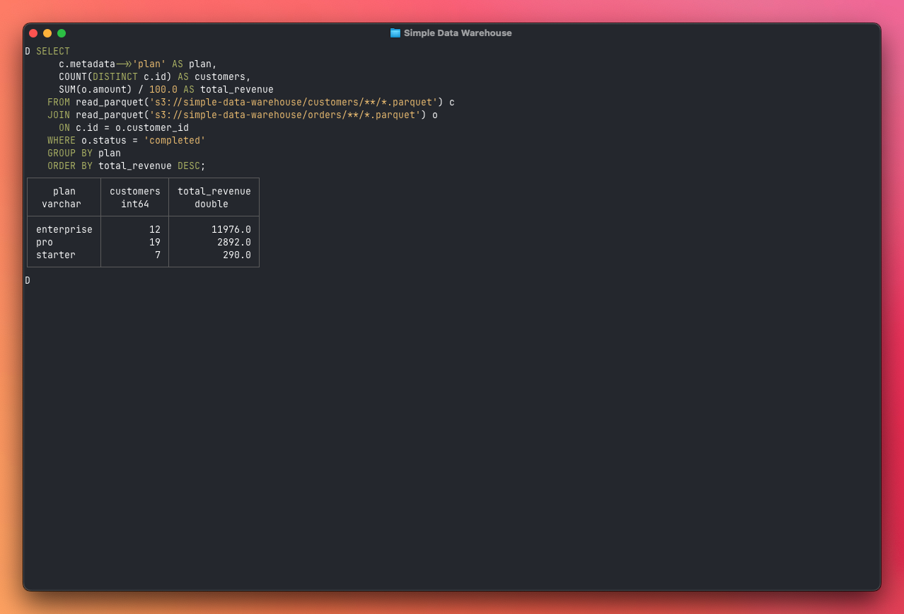
Now let's ask some real questions. The first thing you probably want to know is how revenue breaks down across your customer plans. This query joins customers with orders and extracts the plan from the JSONB metadata field — exactly the kind of cross-source question that's painful to answer against a production database:

SELECT
  c.metadata->>'plan' AS plan,
  count(DISTINCT c.id) AS customers,
  count(o.id) AS orders,
  sum(o.amount) / 100.0 AS total_revenue
FROM customers c
JOIN orders o ON c.id = o.customer_id
WHERE o.status = 'completed'
GROUP BY plan
ORDER BY total_revenue DESC;

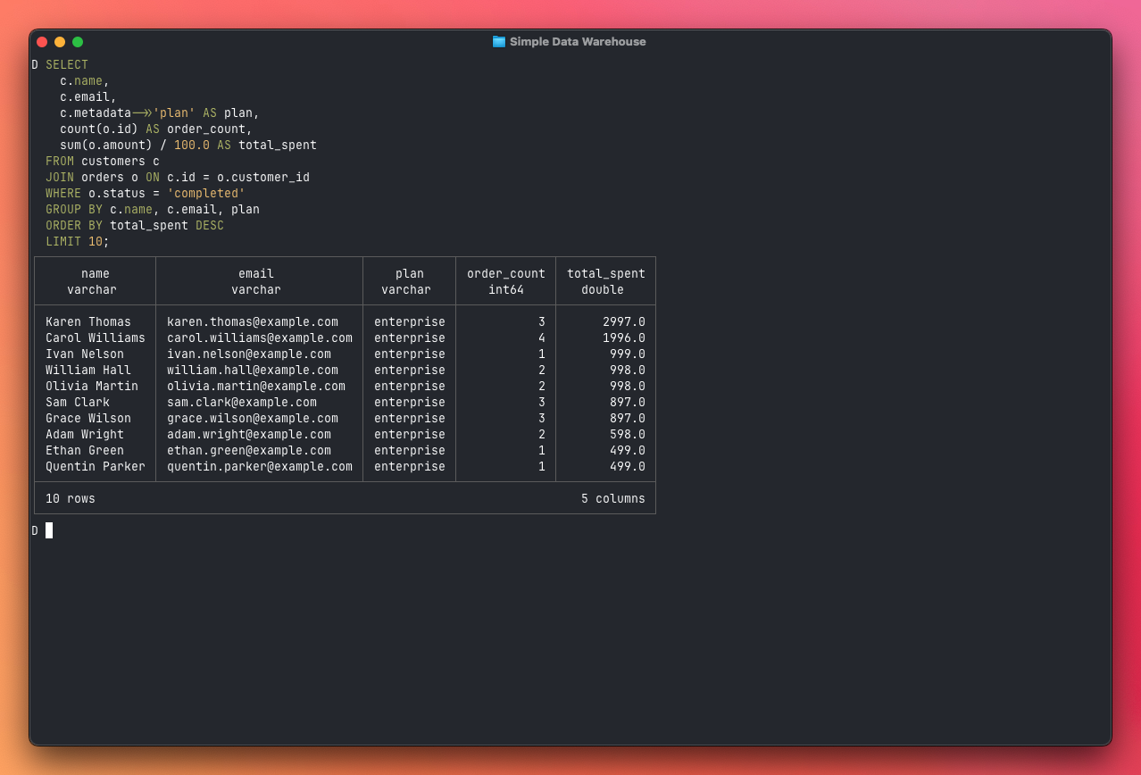
Next, who are your most valuable customers? This is a join between customers and orders, grouped and sorted by total spend:

SELECT
  c.name,
  c.email,
  c.metadata->>'plan' AS plan,
  count(o.id) AS order_count,
  sum(o.amount) / 100.0 AS total_spent
FROM customers c
JOIN orders o ON c.id = o.customer_id
WHERE o.status = 'completed'
GROUP BY c.name, c.email, plan
ORDER BY total_spent DESC
LIMIT 10;

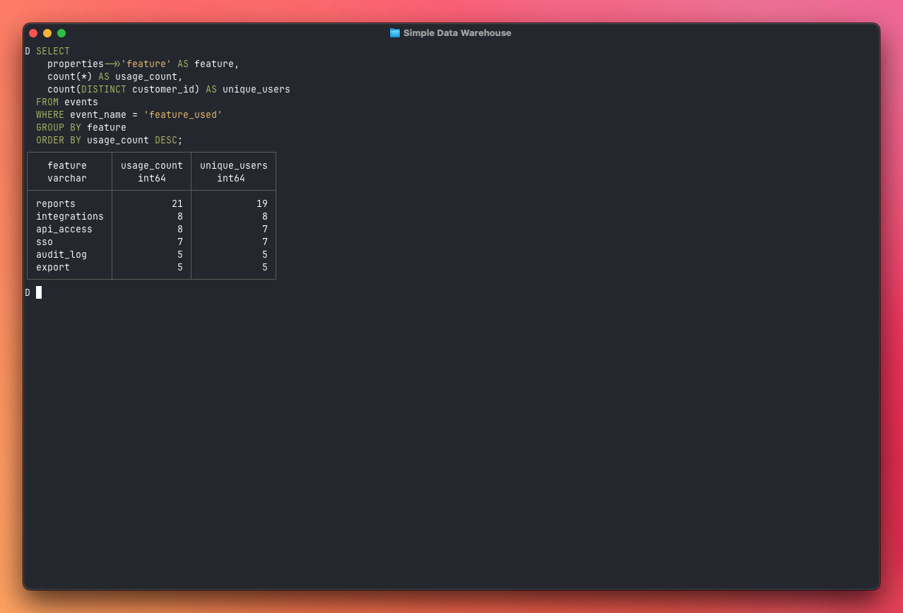
Now things get interesting. The events table lets you understand product usage. Which features are actually getting used, and by how many distinct users?

SELECT
  properties->>'feature' AS feature,
  count(*) AS usage_count,
  count(DISTINCT customer_id) AS unique_users
FROM events
WHERE event_name = 'feature_used'
GROUP BY feature
ORDER BY usage_count DESC;

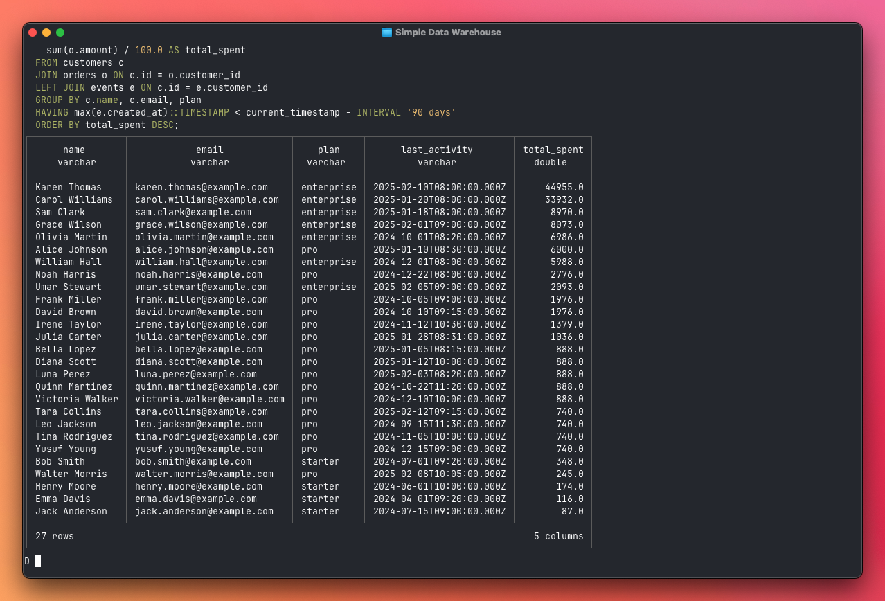
And perhaps the most valuable query for a SaaS business: which paying customers are going quiet? This three-table join finds customers who have spent money but haven't shown any activity in the last 90 days — your churn risk list:

SELECT
  c.name,
  c.email,
  c.metadata->>'plan' AS plan,
  max(e.created_at) AS last_activity,
  sum(o.amount) / 100.0 AS total_spent
FROM customers c
JOIN orders o ON c.id = o.customer_id
LEFT JOIN events e ON c.id = e.customer_id
GROUP BY c.name, c.email, plan
HAVING max(e.created_at)::TIMESTAMP < current_timestamp - INTERVAL '90 days'
ORDER BY total_spent DESC;

All of these queries run entirely on your machine. DuckDB downloads only the columns and partitions it needs, processes them in parallel, and returns results in seconds. No cluster, no warehouse service, no monthly bill. And you can run them from anywhere — a laptop, a CI job, or a Node.js API endpoint — as long as you have access to the S3 bucket.

The repo includes more examples in queries.sql.

Trade-offs and when this breaks down

This architecture works remarkably well for a small team, but it's worth being honest about the limits.

Concurrency. DuckDB is single-process. If two people run heavy queries at the same time against the same DuckDB instance, one waits for the other. In practice this rarely matters because each person runs their own DuckDB process against shared Parquet files on S3. But if you want a shared dashboard with ten concurrent users, you need something like MotherDuck or a traditional warehouse.

Data freshness. This is a batch pipeline. Your warehouse is only as fresh as the last successful run. If you need data updated every few minutes, you'll want a streaming approach — though even then, you can land micro-batches as Parquet files and this architecture still works.

Scale ceiling. DuckDB runs on a single machine. For most SaaS applications, this is fine — even a modest laptop can scan hundreds of millions of rows in seconds. But if you're dealing with billions of rows or terabytes of data, you'll need a distributed engine like ClickHouse, BigQuery, or Snowflake.

No ACID transactions. Overwriting a Parquet file on S3 isn't atomic — there's a brief window where the old file is deleted but the new one isn't fully uploaded. For a daily batch pipeline this is a non-issue, but it's worth knowing if you're thinking about more frequent updates.

Where to go from here

This setup handles a surprisingly large range of use cases. But there are natural extension points when you outgrow it:

More sources. Adding a new data source means writing a new extractor function. Stripe, Hubspot, GitHub — anything with an API can feed into the same pipeline.

Incremental loads. Instead of extracting the full dataset each run, read the last_run_at from your metadata file and only fetch records created or updated since then. The Postgres extractors can add a WHERE updated_at >= $1 clause, and most APIs support similar filtering.

Orchestration. If the pipeline grows beyond three or four extractors, consider a lightweight orchestrator like Inngest or even a simple task queue. This gives you retries, dependency management, and better observability than a simple scheduler.

Self-hosted object storage. The example uses S3, but MinIO is a drop-in S3-compatible replacement you can run on the same machine. DuckDB's httpfs extension works with any S3-compatible endpoint — just set s3_endpoint and s3_url_style = 'path' in your DuckDB config.

The beauty of this architecture is that each piece is independent and replaceable. You can swap S3 for MinIO, replace the scheduler with cron or a proper orchestrator, or upgrade from DuckDB to ClickHouse — all without rebuilding the whole pipeline. Start simple, and add complexity only when you have a specific problem to solve.